Introduction to Q Learning

1. Introduction

Q-learning is a foundational model-free reinforcement learning algorithm. It helps an agent learn the optimal value of actions without needing a detailed model of the environment. The agent’s ultimate goal is to maximize cumulative rewards by learning the best action to take in each state.

1a. How Does It Work?

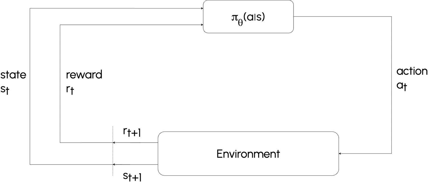
In reinforcement learning, an agent interacts with its environment in discrete steps:

1. Observes the current state $s$.
2. Takes an action $a$.
3. Receives a reward $R(s, a, s')$.
4. Transitions to a new state $s'$

The Q-value, $Q(s, a)$ represents the expected cumulative reward (or return) the agent can achieve by taking action $a$ in state $s$ and then continuing optimally.

2. Understanding Q-Values

Q-values capture the expected utility, or the sum of discounted rewards, starting from state $s$ with action $a$ and then following the optimal policy. This Q-value can be thought of as comprising two parts:

1. The immediate reward for taking action $a$ in state $s$.
2. The discounted future rewards that the agent can expect by following the optimal policy from the next state $s'$.

By continuously updating these Q-values, Q-learning helps the agent gradually approximate the optimal policy, guiding it to take actions that maximize long-term rewards.

2. Bellman Equation for Q values

The relationship between Q-values and future rewards is defined recursively by the Bellman Equation. The Q-value at the next state $s'$ is maximized to choose the best future action:

$$
 Q^*(s, a) = \sum_{s'} P(s' \mid s, a) \left[ R(s, a, s') + \gamma \max_{a'} Q^*(s', a') \right] 
$$

where:

• $Q^*(s, a)$: Optimal Q-value for state $s$ and action $a$.
• $P(s' \mid s, a)$: Probability of transitioning to $s'$ after taking $a$ in $s$.
• $R(s, a, s')$: Immediate reward for the transition.
• $\gamma$ (discount factor): Balances immediate and future rewards.

The Bellman Equation allows us to compute Q-values recursively, helping the agent estimate the total return for any state-action pair.

3. Q-Value Iteration

Q-Value Iteration is a process where Q-values are iteratively updated to converge on the optimal values, Q^*, that guide the agent's decisions. Typically, this process begins with an initial set of Q-values (often initialized to zero) and repeatedly updates them until they converge.

In Q-learning, these updates are based on the following rule:

$$
 Q_{k+1}(s, a) \leftarrow \sum_{s'} P(s' \mid s, a) \left[ R(s, a, s') + \gamma \max_{a'} Q_k(s', a') \right] 
$$

where:

• $Q_k(s, a)$: Current Q-value estimate.
• $Q_{k+1}(s, a)$: Updated Q-value in the next iteration.

Through this iterative process, Q-learning allows the agent to progressively refine its understanding of the optimal action-value function, guiding it toward actions that maximize expected cumulative rewards over time.

4. (Tabular) Q-Learning

Tabular Q-learning is a foundational form of Q-learning that allows an agent to learn directly from actual environment samples, bypassing the need for a complete model of the environment. Instead of computing expectations, it updates Q-values based on observed experiences, making it possible to learn optimal policies even without knowledge of the full transition dynamics.

In tabular Q-learning, actual environment samples replace expectations, allowing agents to learn without a full model. The update can be rewritten as:

$$
 Q_{k+1}(s, a) \leftarrow (1 - \alpha) Q_k(s, a) + \alpha \left[ R(s, a, s') + \gamma \max_{a'} Q_k(s', a') \right] 
$$

4a. Steps for Tabular Q-Learning

1. Initialize all Q-values, usually to zero.

2. The agent begins in an initial state $$s\$$.

3. Choose an action $a$, observe the next state $s'$, and receive reward $R(s, a, s')$.

4. Compute the Target:

   • If $s'$ is terminal: $ \text{target} = R(s, a, s') $

   • Otherwise: $ \text{target} = R(s, a, s') + \gamma \max_{a'} Q_k(s', a') $

5. Update the Q-value with the formula:
   $$
    Q_{k+1}(s, a) \leftarrow (1 - \alpha) Q_k(s, a) + \alpha \cdot \text{target} 
   $$
   

where:

• $\alpha$: Learning rate (how much new information influences Q-values).
• $\gamma$: Discount factor (weights future rewards).

5. Applications and Limitations