1. Introduction
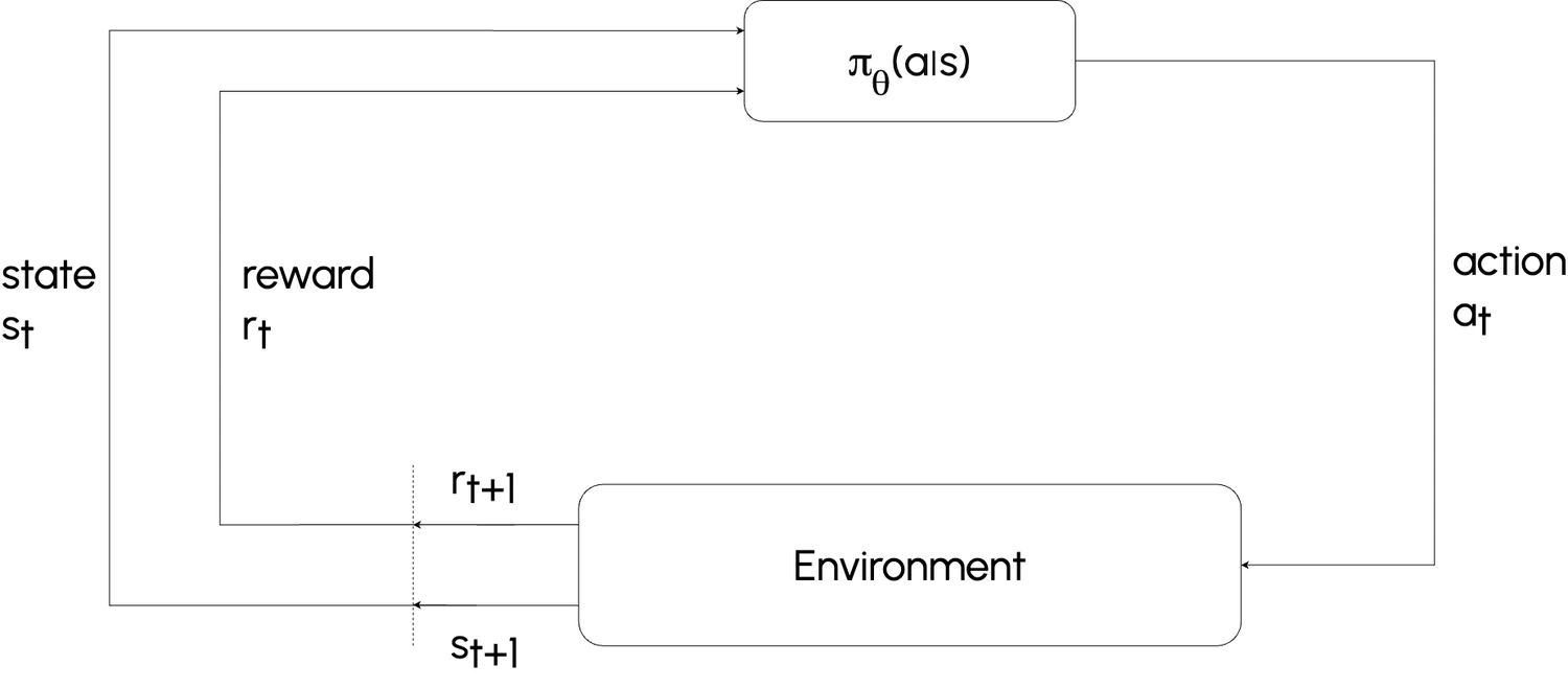
In this lesson, we explore the transition from using a Q-table to employing a parameterized Q-function , typically represented by a neural network, to estimate Q-values. This shift is crucial for handling environments with continuous or high-dimensional state-action spaces , where storing explicit Q-values for every state-action pair is infeasible.We’ll dive into how neural networks approximate Q-values, introducing key concepts like target networks and replay buffers , which are critical for stabilizing training and ensuring effective learning.
2. Learning Process

2a. Generating a Target
When the agent transitions from state $s$ to $s'$ after taking action $a$, it receives a reward $R(s, a, s')$. The target value for the Q-function combines this immediate reward with the discounted future reward:
$$
\text{target}(s') = R(s, a, s') + \gamma \max_{a'} Q_{\theta_k}(s', a')
$$
where:
-
$\gamma$: Discount factor, balancing immediate and future rewards.
-
$\max_{a'} Q_{\theta_k}(s', a')$: Estimated future reward from the next state $s'$, calculated using the current Q-function $Q{\theta_k}$.
2b. Updating Parameters $\theta$
Unlike tabular Q-learning, where Q-values are directly updated, Approximate Q-Learning uses gradient descent to adjust the parameters $\theta$ of the neural network. The goal is to minimize the difference between the predicted Q-value $Q_{\theta}(s, a)$ and the target value.
2c. Objective Function
The loss function measures the error between the predicted Q-value and the target value:
$$
L(\theta) = \frac{1}{2} \left( Q_{\theta}(s, a) - \text{target}(s') \right)^2
$$
The network parameters are updated via gradient descent:
$$
\theta_{k+1} \leftarrow \theta_k - \alpha \nabla_\theta L(\theta) \bigg|_{\theta = \theta_k}
$$
where $\alpha$ is the Learning rate.
2d. Iterative Learning
To prevent overfitting to individual experiences, the network is trained iteratively using a diverse set of experiences, allowing the Q-function $Q_{\theta}$ to improve incrementally as it encounters new states and actions.
3. Deep Q-Network (DQN) Training Algorithm
Deep Q-Networks (DQNs) are a specific implementation of Approximate Q-Learning, leveraging replay buffers and target networks to stabilize and enhance training. The core steps of the algorithm are as follows:
3a. Replay Buffer
A replay buffer $D$ stores past experiences $(s_t, a_t, r_t, s_{t+1})$, enabling the agent to learn from a diverse set of transitions rather than consecutive, highly correlated experiences:
$$
D = \{ (s_t, a_t, r_t, s_{t+1}) \}
$$
The buffer has a fixed size, discarding the oldest experiences as new ones are added.
3b. Q-Function Parameterization
The Q-function is approximated by a neural network $Q(s, a; \theta)$, referred to as the main Q-network . To stabilize training, a separate target Q-network $\hat{Q}(s, a; \theta^-)$ is used, with parameters $\theta^-$ updated periodically to match $\theta$.
$$
Q(s_t, a_t; \theta) \quad (\text{Main Q-network})
$$
$$
\hat{Q}(s_t, a_t; \theta^-) \quad (\text{Target Q-network})
$$
3c. Action Selection (Epsilon-Greedy Policy)
The agent selects actions using an epsilon-greedy policy :
-
With probability $\epsilon$, the agent explores by choosing a random action.
-
With probability $1 - \epsilon$, the agent exploits by selecting the action with the highest Q-value:
$$
a_t =
\begin{cases}
\text{random action} & \text{with probability } \epsilon \\
\arg \max_a Q(s_t, a; \theta) & \text{with probability } 1 - \epsilon
\end{cases}
$$
3d. Storing Transitions in Replay Buffer
After executing action $a_t$, the agent observes the reward $r_t$ and next state $s_{t+1}$. This transition is stored in the replay buffer $D$:
$$
D \leftarrow D \cup (s_t, a_t, r_t, s_{t+1}).
$$
3e. Sampling from Replay Buffer
A mini-batch of transitions is randomly sampled from the replay buffer for training. Sampling randomly breaks correlations between consecutive experiences, improving training stability.
$$
\{ (s_j, a_j, r_j, s_{j+1}) \}_{j=1}^N \sim D
$$
3f. Computing Target Values
For each transition in the mini-batch, compute the target value $y_j$.
-
If $s_{j+1}$ is terminal, the target is the reward $r_j$.
-
Otherwise, the target includes the discounted maximum Q-value from the target network:
$$
y_j = \begin{cases} r_j & \text{if } s_{j+1} \text{ is terminal}, \\ r_j + \gamma \max_{a'} \hat{Q}(s_{j+1}, a'; \theta^-) & \text{otherwise}. \end{cases}
$$
Where $ \gamma $ is the discount factor.
3g. Loss Function
The objective is to minimize the difference between the predicted Q-value $ Q(s_j, a_j; \theta) $ and the target value $y_j$ (computed in the previous step). The loss function is the mean squared error between these two quantities:
$$ L(\theta) = \frac{1}{N} \sum_{j=1}^{N} \left( y_j - Q(s_j, a_j; \theta) \right)^2. $$
3h. Gradient Descent
Perform a gradient descent step to update the Q-network parameters $\theta$ by minimizing the loss $L(\theta)$. The gradient of the loss with respect to $\theta$ is computed and used for updating:
$$
\theta \leftarrow \theta - \alpha \nabla_\theta L(\theta)
$$
Where $\alpha$ is the learning rate.
3i. Updating the Target Network
Every $C$ steps, the target network’s parameters $\theta^-$ are updated to match the main Q-network’s parameters $\theta$. This periodic update helps stabilize learning by decoupling the target computation from the rapidly changing Q-network:
$$ \theta^- \leftarrow \theta. $$
This concludes the step-by-step breakdown of the Deep Q-Network (DQN) training algorithm.
4. Summary
This lesson introduced the mechanics of Approximate Q-Learning, with a focus on the Deep Q-Network (DQN) algorithm. Key innovations like replay buffers, target networks, and epsilon-greedy action selection address challenges of instability and inefficiency in training, enabling reinforcement learning agents to operate in complex, high-dimensional environments.
Sources
-
Foundations of Deep RL by Pieter Abbeel
-
Full implementation: Deep Q-Learning on GitHub